Disclaimer: This article is for educational purposes only. It summarises working-paper research that has not been peer reviewed. Trading and investments are subject to volatility, market risks, and macroeconomic shifts that could lead to partial or total loss of capital. Nothing here is investment advice or a recommendation to use any model in a live risk or trading system. Please consult your own risk, compliance and investment professionals before acting on any of it.
Financial Gurkha | Research Note | September 26, 2026
By Niraj Neupane, CA (ICAI), Quantitative Researcher. This article applies the author's own working paper, Conditional Tail Episode Risk, to this week's Treasury selloff. The paper is available in full on SSRN.

On Wednesday, September 23, the U.S. Treasury market had its worst day in a year and a half. The 10-year yield rose more than 13 basis points Basis point (bp)One hundredth of a percentage point. A 13 bp rise takes a yield from 4.97% to 5.10%. to about 5.10%, its biggest one-day move in nearly 18 months and its highest level since July 2007. By Friday it had reached 5.23%.
Most coverage focused on that single day, and in most risk systems that single day is what gets measured. A 99% one-day Value-at-Risk Value-at-Risk (VaR)The loss threshold a portfolio is not expected to exceed on a given day at a chosen confidence level. A 99% one-day VaR of $10 million means losses above $10 million should happen on about 1 day in 100. number is recalculated, a limit is checked, and the day is marked as a breach or not.
That framing misses how this week actually unfolded. The damage came from a sequence: a strong growth report, a weak auction, rising rate-hike odds, another soft auction, and higher yields again. Each step fed the next. In risk terms it was an episode, a connected run of extreme losses. Our standard risk measures are built to size individual days, and they cannot tell an episode apart from the same bad days scattered across a quarter.
SSRN Working Paper, September 2026 · Abstract 7502499
Conditional Tail Episode Risk: A Path-Dependent Framework for Extreme-Loss Episodes Beyond Value-at-Risk and Expected Shortfall
Niraj Neupane
Proposes Tail Episode Risk (TER), the upper-tail quantile of the worst connected run of extreme losses over a finite horizon, and Conditional TER (CTER), which splits episode risk into the probability of entering an episode and its conditional severity. Tested by simulation, constructed stress scenarios, and 2000 to 2026 data on the S&P 500, Nasdaq, long-duration Treasuries, EUR/USD, USD/JPY and Bitcoin.
The 60-Second Version#↑ Contents
| What | Number |
|---|---|
| 10-year Treasury yield, Friday | 5.23%, highest since 2007 |
| Wednesday's move | +13 bp, largest in ~18 months |
| Rise since the start of 2026 | +108 bp (from 4.15%) |
| Estimated loss on a par 10-year since January | about 8% of price |
| Episode risk when losses cluster (simulation) | ~3× higher, with VaR/ES flat |
| Best episode-forecasting market of six tested | Treasuries (AUC 0.64 at 99%) |
| Did the richer CTER model beat simple EWMA? | No |
The seven things that matter:
- This week was a run, not a shock. A hot services PMI, a weak 5-year auction, a 13 bp jump, a soft 7-year auction and a 5.23% close all fed each other over five sessions.
- VaR and Expected Shortfall ignore the order of losses. Three bad days in a row and three bad days spread over a quarter produce the same VaR and the same ES.
- Tail Episode Risk (TER) measures the run. It groups consecutive extreme-loss days into episodes, sums how far each day exceeded the threshold, and takes the tail of the worst episode over a 10-day horizon.
- Clustering can triple episode risk while VaR and ES stay flat. In simulation, 99% TER rose from 1.51 to 4.54 as serial dependence rose. VaR and ES barely moved.
- The two views can disagree on which scenario is riskier. A sustained liquidity collapse scored 12.00 on episode severity against 3.50 for scattered spikes that VaR and ES ranked higher.
- Bond-market episodes are the most predictable of six markets tested. Long-duration Treasuries held an AUC of 0.64 to 0.67 even in the deep tail. Equities, currencies and Bitcoin faded toward a coin flip or below.
- The honest result: more features did not help. The full CTER conditioning set forecast episode severity worse than a simple EWMA volatility model at the 95% and 97.5% thresholds, and no better at 99%.
What's in this report#
- The 60-Second Version
- 1. The Week in Numbers
- 2. The Blind Spot in VaR and Expected Shortfall
- 3. What Is Tail Episode Risk (TER)?
- 4. What the Research Found, Good and Bad
- 5. Why a Negative Result Is Still Useful
- 6. Why Episode Risk Matters for the U.S. Financial System
- 7. What Risk Managers Can Do Now
- 8. Limitations and What Comes Next
- Frequently Asked Questions
- Conclusion and Key Takeaways
- Methodology and Sources
1. The Week in Numbers#↑ Contents
Market figures below are as reported by CNBC, CNN Business, NBC News and others for the week of September 21 to 25, 2026. Full links are in Methodology and Sources.
| Indicator | Level / move | Why it matters |
|---|---|---|
| 10-year Treasury yield | 5.23% (Friday), up from 4.15% at the start of 2026 | Highest since 2007; the benchmark for mortgages and corporate borrowing |
| Wednesday's 10-year move | +13 bp to ~5.10% | Largest one-day jump in ~18 months |
| 2-year Treasury yield | ~4.87% to 4.90% | Highest since 2024; signals expected Fed tightening |
| 30-year Treasury yield | ~5.4% | Highest since before the 2008 financial crisis |
| Fed funds target | 3.75% to 4.00% | First hike in three years, on September 16 |
| October hike odds (CME FedWatch CME FedWatchA tool from CME Group that converts fed funds futures prices into the market-implied probability of each possible Fed decision at upcoming meetings.) | ~64% | Markets expect more tightening |
| S&P Global services PMI PMI (Purchasing Managers' Index)A monthly survey of business activity. Readings above 50 mean activity is expanding; the further above 50, the faster the expansion. | 58.7 (from 56.5) | Strongest in nearly five years |
| 5-year and 7-year auctions Weak Treasury auctionAn auction is called weak when investors demand a higher yield than the market was trading just before the sale (a "tail") or bid for fewer bonds than usual. It signals that new supply is hard to place. | Weak / soft demand | Supply pressure on the curve |
| WTI–10yr correlation (1-month) | 0.96 (BMO) | Oil and rates moving almost in lockstep |
| 30-year mortgage rate | above 7.2% in daily lender surveys | A one-year high for household borrowing costs |
| Michigan 1-yr inflation expectations | 4.6% (from 4.0%) | Highest since June |
| S&P 500 (Friday close) | 7,743.41 | Winning week after a three-day losing streak |
1.1 How the week's losses fed on each other#
Read in order, the week was a chain, and every link raised the odds of the next:
- Hot growth data. The S&P Global services PMI printed 58.7, its strongest in nearly five years.
- Rate-hike odds rise. Markets priced roughly a 64% chance of another Fed hike in October.
- A weak 5-year auction showed buyers demanding more yield to absorb new supply.
- The 10-year jumps 13 bp on Wednesday, the largest one-day move in about 18 months.
- A soft 7-year auction the next day added pressure rather than relief.
- The 10-year reaches 5.23% on Friday.
Running underneath all six steps was oil. With the Iran war keeping crude elevated, the one-month correlation between WTI and the 10-year yield reached 0.96, according to BMO. Higher oil fed inflation expectations, which fed hike odds, which fed yields. The last step then becomes the first step of whatever comes next.
1.2 What that means for a bond portfolio#
A 10-year Treasury near a 5.2% yield has a modified duration Modified durationThe approximate percentage change in a bond's price for a one-percentage-point change in its yield. A duration of 7.7 means a 1% rise in yield cuts the price by about 7.7%. of about 7.7. For a par bond paying semiannually, modified duration is (1 − 1.026⁻²⁰) ÷ 0.052 ≈ 7.72.
| Move | Yield change | Approx. price impact | Loss on $10B of 10-yr-equivalent |
|---|---|---|---|
| Start of 2026 → now | ≈ +108 bp | ≈ −8% | ≈ $800M |
| Early September → now | ≈ +45 bp | ≈ −3.4% | ≈ $340M |
The arithmetic: −7.72 × 1.08% = −8.3%, plus a small convexity ConvexityThe curvature in the price-yield relationship. It means a bond loses a little less than duration alone predicts when yields rise, and gains a little more when they fall. offset of about +0.4%, gives roughly −8%. For the 45 bp move, −7.72 × 0.45% = −3.5%, plus about +0.1% convexity, gives roughly −3.4%. These are first-order illustrative estimates, not reported figures.
Equities held up surprisingly well. The S&P 500 recovered from a three-day losing streak to finish the week higher. That resilience is why this story is easy to miss. Nothing crashed, but pressure built up over several days.
2. The Blind Spot in VaR and Expected Shortfall#↑ Contents
VaR and Expected Shortfall measure how bad individual days are, not how bad days line up. Both are calculated from the marginal distribution of losses, the set of daily outcomes without regard to the order they arrive in.
The two are the main tools of market risk measurement. VaR gives the loss threshold you are unlikely to exceed at a chosen confidence level. Expected Shortfall Expected Shortfall (ES)The average loss on the days that are worse than VaR. If 97.5% VaR is $10 million, 97.5% ES is the average of all losses larger than $10 million. It captures how deep the tail goes, not just where it starts. averages the losses beyond that threshold. Under Basel's Fundamental Review of the Trading Book FRTB (Fundamental Review of the Trading Book)The Basel Committee's framework for how much capital banks must hold against trading-book market risk. It replaced 99% VaR with 97.5% Expected Shortfall as the core capital measure., ES is now the core measure of regulatory market-risk capital.
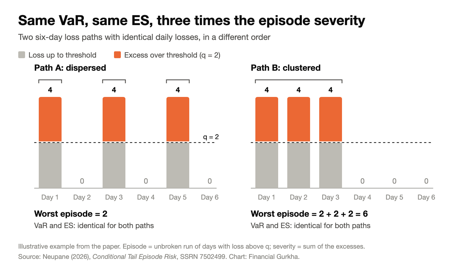
A simple example shows the problem. Take two six-day loss paths with a tail threshold of 2:
| Day | 1 | 2 | 3 | 4 | 5 | 6 | VaR / ES | Worst-episode severity |
|---|---|---|---|---|---|---|---|---|
| Path A (dispersed) | 4 | 0 | 4 | 0 | 4 | 0 | Identical | 2 |
| Path B (clustered) | 4 | 4 | 4 | 0 | 0 | 0 | Identical | 6 |
Both paths contain three losses of 4 and three zeros, so their VaR and ES are identical. Path A has three separate one-day episodes, each with an excess of 4 − 2 = 2. Path B has one continuous episode with a cumulative excess of 2 + 2 + 2 = 6, three times larger.
This matters because the damage that breaks institutions is usually sequential:
- Funding and margin stress builds with consecutive losses, since collateral calls compound before assets can be sold.
- Forced selling feeds on itself when each day's loss triggers the next day's liquidation.
- Depositor and investor confidence reacts to how long bad news lasts, not only to one headline.
Silicon Valley Bank in 2023 is the clearest recent example. The bank did not fail because of one bad bond-market day. It failed because a long run of rising rates built up unrealized losses on its securities portfolio faster than any daily risk number showed, until depositors noticed.
3. What Is Tail Episode Risk (TER)?#↑ Contents
Tail Episode Risk (TER) is the upper-tail quantile of the worst connected run of extreme losses over a fixed horizon. Where VaR asks how large one bad day can be, TER asks how severe the worst unbroken streak of bad days can become. It was proposed in the working paper Conditional Tail Episode Risk (SSRN, September 2026).
3.1 How TER is built, in three steps#
- Set a tail threshold. Any day whose loss exceeds a high quantile, such as the 95th percentile, counts as extreme.
- Group extreme days into episodes. An episode is an unbroken run of consecutive extreme days. Its severity is the sum of how far each day in the run exceeded the threshold.
- Take the worst episode, then its tail. Over a horizon (10 trading days in the study), find the most severe episode, called S*. TER is the upper-tail quantile of that worst-episode severity.
In formula terms, with daily losses L, threshold q at level α, tail level β, horizon H and information at time t:
TER  = Q_β [ max over episodes j of  Σ (L_t+k − q_t,α)⁺  for k in j  |  information at t ]

CTER = P( an episode occurs in the next H days | X_t )      <- how likely?
     × ES_β( S*_t,H | an episode occurs, X_t, Z_t )          <- how bad?
3.2 Conditional TER: how likely, and how bad?#
Conditional Tail Episode Risk (CTER) splits episode risk into the probability of entering an extreme-loss episode and the expected severity of that episode if it happens, both conditioned on current market conditions. Those are the two questions a risk committee actually asks:
How likely are we to enter an extreme-loss episode, given current conditions? > If we do, how bad could it get?
A risk report that today says "VaR 5%, ES 7%" could add an episode probability and an episode severity next to them.
3.3 How TER compares with VaR, ES and drawdown#
| Measure | Question it answers | Depends on order of losses? | Sensitive to clustering? | Status |
|---|---|---|---|---|
| VaR | How large is the loss threshold? | No | No | Existing |
| ES | How severe is the marginal tail? | No | No | Existing (Basel FRTB) |
| Aggregate excess | How much total exceedance occurs in an extreme event? | Event-level | Yes | Prior art (Anderson, 1994) |
| Conditional Expected Drawdown DrawdownThe fall from a portfolio's previous peak to a later low. Conditional Expected Drawdown averages the worst drawdowns, the way ES averages the worst days. | How deep can a peak-to-trough decline get? | Yes | Yes | Related |
| TER | How severe can the worst connected run of extreme losses become? | Yes | Yes | Proposed |
| CTER | Given today's conditions, how likely and how severe is that run? | Yes | Yes | Proposed |
What the paper does not claim. Summing threshold exceedances is established extreme value theory Extreme value theory (EVT)The branch of statistics that models rare, extreme outcomes, such as the largest losses in a series, rather than typical ones., and the mathematics of extreme clusters is well developed. The contribution is turning the worst episode over a finite horizon into a conditional forecast target for financial risk, splitting it into probability and severity, and testing it with modern forecast-evaluation standards. The paper also proves TER is not a disguised drawdown measure: the two can rank the same paths in opposite order.
4. What the Research Found, Good and Bad#↑ Contents
The framework was tested three ways: controlled simulation, deliberately constructed stress scenarios, and 26 years of real data (2000 to 2026) across six markets: the S&P 500, Nasdaq, long-duration Treasuries (TLT TLTThe iShares 20+ Year Treasury Bond ETF, a widely traded fund holding long-maturity U.S. Treasuries. Its daily returns are a standard proxy for long-duration bond risk.), EUR/USD, USD/JPY and Bitcoin.
| # | Question | Result | Verdict |
|---|---|---|---|
| 1 | Does clustering raise episode risk when VaR/ES stay flat? | 99% TER rises ~3× while VaR/ES barely move | Yes |
| 2 | Can VaR/ES and TER disagree on which scenario is riskier? | Liquidity collapse: VaR 3.5 but S* 12.0 | Yes |
| 3 | Does episode severity identify real crises? | Flags 2020, 2008, 2025, 2011, 2000–02 | Yes |
| 4 | Can episodes be predicted in advance? | Weak overall; bonds are the exception (AUC 0.64 to 0.67) | Mixed |
| 5 | Does CTER's richer feature set beat a simple volatility model? | No. Worse at 95% and 97.5%, no difference at 99% | No |
4.1 Clustering can triple episode risk while VaR and ES stay flat#
The paper simulated return series with the same marginal distribution and increased only the serial dependence Serial dependence (ρ)How strongly one day's outcome is linked to the previous day's. At ρ = 0 each day is independent; at ρ = 0.9 a bad day is very likely to be followed by another. ρ.
| Serial dependence ρ | VaR 95% | ES 95% | TER 95% | TER 99% |
|---|---|---|---|---|
| 0.0 | 1.633 | 2.059 | 0.981 | 1.508 |
| 0.3 | 1.645 | 2.053 | 1.010 | 1.737 |
| 0.7 | 1.655 | 2.046 | 1.065 | 2.580 |
| 0.9 | 1.668 | 2.093 | 1.060 | 4.541 |
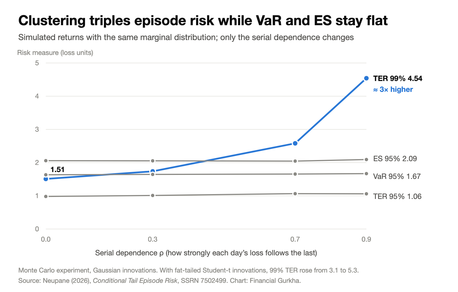
VaR and ES barely moved, while 99% TER rose 3.0× (4.541 ÷ 1.508). With fat-tailed, variance-standardized Student-t innovations, the pattern held: 99% TER rose from 3.1 to 5.3.
Takeaway: loss clustering, the defining feature of a week like this one, can sharply increase episode risk while the headline risk numbers stay the same.
4.2 VaR/ES and TER can rank the same scenarios in opposite order#
The paper constructed six 60-day stress paths with a common, fixed threshold (q = 2.5).
| Scenario | VaR 95% | ES 95% | Worst-episode severity S* | Which looks riskier? |
|---|---|---|---|---|
| Isolated crash | 1.42 | 4.00 | 6.50 | |
| Tail thickening (isolated spikes) | 6.00 | 6.00 | 3.50 | VaR/ES say this one |
| Liquidity collapse (sustained run) | 3.50 | 3.50 | 12.00 | TER says this one |
| Volatility explosion (cluster) | 6.42 | 7.68 | 25.62 | Both agree |
| Broad contagion (all elevated) | 3.39 | 4.01 | 2.40 | Neither captures it well |
| Escalating deterioration | 3.58 | 4.52 | 7.80 |
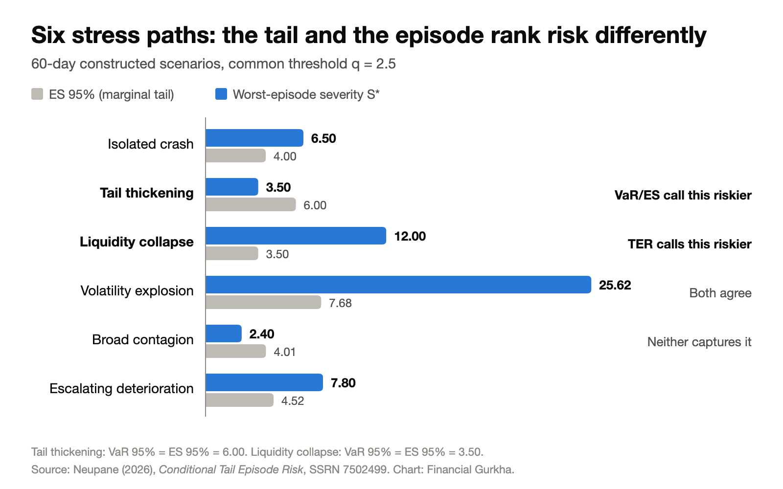
VaR and ES say the scattered-spikes scenario is riskier. TER says the sustained liquidity collapse is 3.4 times worse by episode severity (12.00 ÷ 3.50). Neither is simply correct. They capture different dimensions of stress, and a risk system tracking only one misses the other.
4.3 The measure identifies real crises#
Applied to realized S&P 500 losses from 2000 to 2026 (10-day horizon), the most severe distinct episodes line up with the periods practitioners remember as crises:
| Rank | Episode | Context |
|---|---|---|
| 1 | March 2020 | COVID crash (10-day worst-episode severity 11.3%) |
| 2 | October to November 2008 | Global financial crisis |
| 3 | March 2025 | Selloff |
| 4 | August 2011 | U.S. downgrade and euro crisis |
| 5 | 2000 to 2002 | Dot-com unwind |
4.4 Bonds are where episodes are most predictable#
The paper tested whether current conditions could forecast whether an episode would occur over the next 10 days. The conditioning set was the VIX, realized volatility, drawdown, the Chicago Fed NFCI NFCI (National Financial Conditions Index)A weekly Chicago Fed index of U.S. financial conditions across money markets, debt, equity and banking. Positive readings mean tighter than average conditions., the St. Louis Fed Financial Stress Index St. Louis Fed Financial Stress IndexA weekly index built from 18 interest rates, yield spreads and other indicators. Zero is normal; positive readings indicate above-average financial stress., and recent episode behavior. AUC AUC (area under the ROC curve)A score for how well a model separates events from non-events. 0.5 is a coin flip, 1.0 is perfect, and below 0.5 is worse than guessing. measures that ability.
| Asset | AUC @ 95% | AUC @ 97.5% | AUC @ 99% | Read |
|---|---|---|---|---|
| S&P 500 | 0.563 | 0.471 | 0.405 | Fades in the tail |
| Nasdaq | 0.563 | 0.519 | 0.423 | Fades in the tail |
| TLT (20+ yr Treasuries) | 0.672 | 0.664 | 0.644 | Holds up in the tail |
| EUR/USD | 0.597 | 0.601 | 0.467 | Fades at 99% |
| USD/JPY | 0.599 | 0.581 | 0.473 | Fades at 99% |
| Bitcoin | 0.377 | 0.427 | 0.403 | Below random |
| Cross-asset mean | 0.56 | 0.54 | 0.47 | Weak overall |
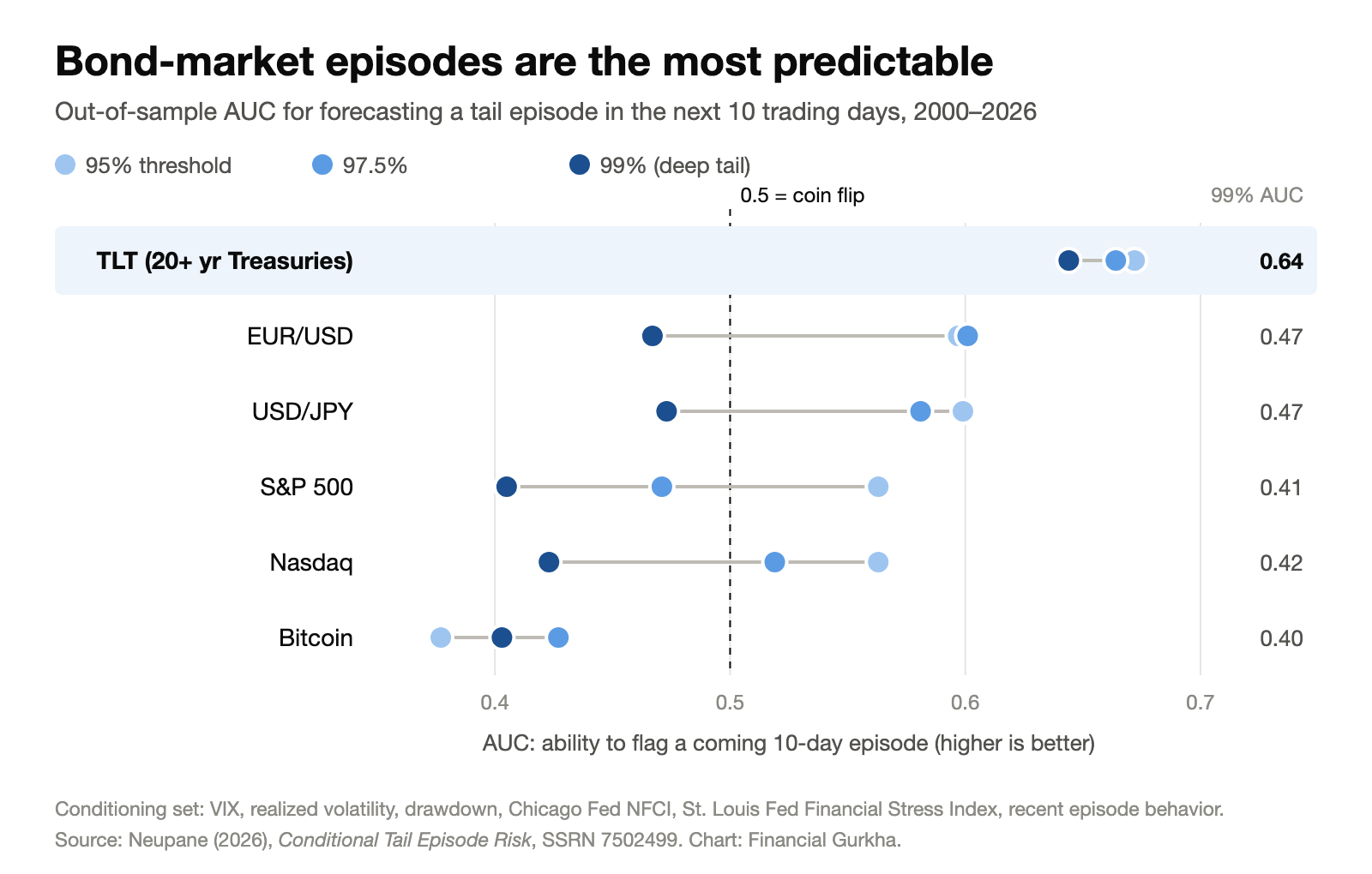
In equities, currencies and Bitcoin, predictability faded as the threshold rose. In long-duration Treasuries it held up, even in the deep tail.
This is consistent with the week's pattern. Treasury stress tends to build through observable steps: inflation data, auction results, Fed communication and term premium Term premiumThe extra yield investors demand for holding a long-term bond instead of rolling over short-term ones. It rises when investors worry about inflation, supply or uncertainty.. That gives risk managers something to monitor. Bond episodes build in ways that show up in the data, and our measures should be designed to see them.
4.5 The forecasting layer did not beat a simple baseline#
This is the result most papers would bury, and the most important one to state plainly.
The paper tested whether the full CTER conditioning set improved episode-severity forecasts over a simple EWMA volatility baseline EWMA (exponentially weighted moving average)A volatility estimate that weights recent returns more heavily than older ones. Popularised by J.P. Morgan's RiskMetrics in the 1990s, it is simple, fast and hard to beat.. Both used the same gradient-boosted estimator and the same walk-forward protocol with a purge gap Walk-forward with purge gapA backtest that trains only on past data, forecasts the next period, then rolls forward. The purge gap drops observations between training and test windows so overlapping horizons cannot leak future information into the model., so there was no look-ahead.
| Threshold | MAE difference (CTER − baseline) | 95% block-bootstrap CI Block bootstrapA resampling method that draws whole blocks of consecutive days rather than single days, so the confidence interval respects the clustering in financial data. | Diebold–Mariano p Diebold–Mariano testA standard statistical test of whether two forecasting models have significantly different accuracy. A small p-value means the gap is unlikely to be chance. | Verdict |
|---|---|---|---|---|
| 95% | +0.00123 | [+0.00073, +0.00179] | below 0.001 | CTER significantly worse |
| 97.5% | +0.00072 | [+0.00034, +0.00114] | below 0.001 | CTER significantly worse |
| 99% | +0.00017 | [−0.00008, +0.00041] | 0.077 | No significant difference |
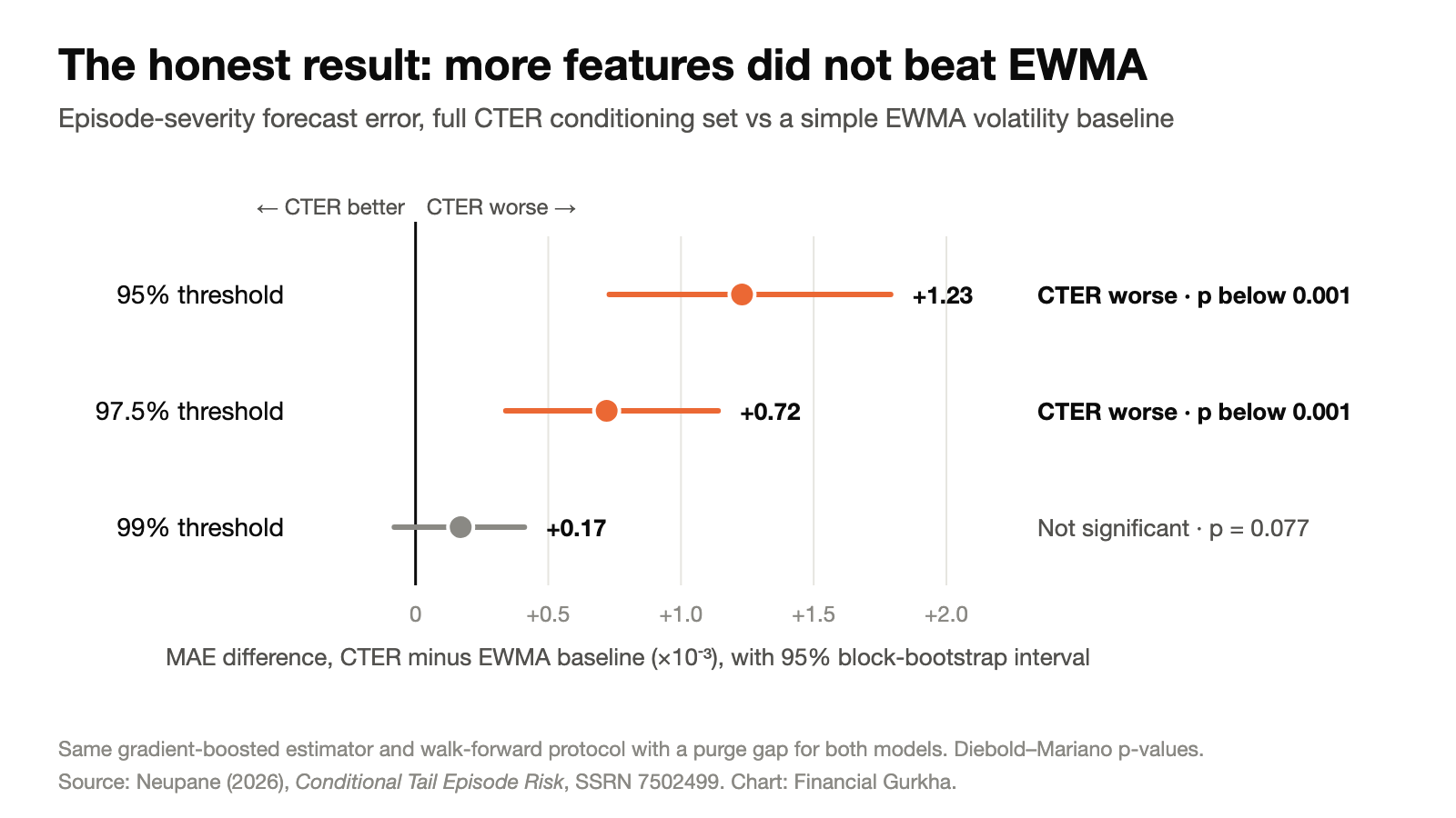
The result held across horizons from 5 to 60 days, across five threshold levels, and under four scoring approaches: point MAE, TER pinball loss Pinball lossThe standard scoring rule for quantile forecasts. It penalises misses asymmetrically according to the quantile being forecast, so it rewards being close, not just avoiding breaches., a Fissler–Ziegel severity score, and a parametric extreme-value model.
| Robustness check | Range tested | Did conditioning help? |
|---|---|---|
| Horizon | H = 5, 10, 20, 60 days | No; the gap widens at longer horizons |
| Threshold | α = 90% to 99% | No; significantly worse everywhere except 99% |
| Scoring rule | MAE, pinball, Fissler–Ziegel | No systematic gain under any |
| Estimator | Gradient boosting and conditional GPD GPD (generalized Pareto distribution)The distribution extreme value theory uses to model losses beyond a high threshold. A conditional GPD lets its parameters move with market conditions. | Better on typical episodes, worse on deep-tail ones |
Conclusion: over 2000 to 2026, adding more market-state information did not improve episode forecasts over a simple volatility model. More variables added estimation noise without enough extra signal.
5. Why a Negative Result Is Still Useful#↑ Contents
A risk measure can capture something real and still be hard to forecast. The paper separates those two questions and answers them differently:
| Question | Answer | Evidence |
|---|---|---|
| Does TER measure something VaR and ES miss? | Yes | Theory, simulation, stress tests, crisis history |
| Does CTER's conditional layer forecast better than simple models? | Not yet | Out-of-sample tests across six markets, 2000 to 2026 |
Put as a pipeline, risk functional → target → estimator → forecast → decision, the research supports the first two links. The estimator, forecast and decision links are still open.
This distinction matters beyond academia. Financial institutions are adopting AI-driven risk models quickly, and a model with more features and more complexity can look more impressive while forecasting worse. Under the Federal Reserve's SR 11-7 SR 11-7The Federal Reserve and OCC's 2011 supervisory guidance on model risk management. It requires banks to validate models independently, document their limitations and govern how they are used. model risk guidance, complexity is not evidence of quality. This result shows why: a sophisticated conditioning layer lost to EWMA, a model from the 1990s.
The framework is also designed to be auditable:
| Object | Elicitable? ElicitableA risk measure is elicitable if some scoring function is minimised by the correct forecast. That is what makes it possible to backtest and compare models objectively. VaR is elicitable; ES alone is not, but VaR and ES together are. | How to backtest it |
|---|---|---|
| TER | Yes | Pinball loss plus a coverage test; model-free, like VaR |
| CTER (as one number) | No (proved by counterexample) | Evaluate in parts |
| CTER: episode probability | Yes | Brier score Brier scoreThe mean squared error of probability forecasts. Lower is better; it rewards forecasts that are both confident and correct. / AUC |
| CTER: episode severity | Yes (jointly) | Fissler–Ziegel score, as with VaR/ES |
That gives supervisors and model validators a clear evaluation protocol rather than a black box.
6. Why Episode Risk Matters for the U.S. Financial System#↑ Contents
Episode risk is not only a quant's concern. Weeks like this one test four parts of the U.S. economy.
| Channel | This week's evidence | Why episode risk matters |
|---|---|---|
| 1. Bank balance sheets | Unrealized losses on bank securities portfolios grow as yields climb | Unrealized losses and deposit flight both build over episodes, as at SVB |
| 2. Housing affordability | 30-year mortgage rates above 7.2% in daily lender surveys | A sustained rise feeds into what millions of households pay; one volatile day that reverses does not |
| 3. Public finance | Weak 5-year and 7-year auctions | Consecutive weak auctions raise the cost of financing the national debt in steps |
| 4. Cross-market contagion | WTI–10yr correlation of 0.96 | Energy and rates now fail together, so a single-asset measure misses joint episodes |
The fourth channel points directly to the next step in this research. In the stress tests, the broad contagion scenario, where all assets are moderately elevated, produced low single-asset episode severity (S* = 2.40), even though it is exactly the kind of systemic stress regulators care about. For more on how oil and the dollar have moved together since 2022, see our DXY, gold and oil analysis.
7. What Risk Managers Can Do Now#↑ Contents
| # | Action | Why |
|---|---|---|
| 1 | Report episodes alongside days. Add realized worst-episode severity over rolling 10-day windows to VaR/ES reports. | It can be computed after the fact with no model |
| 2 | Backtest the clustered-loss periods. Check model behavior across connected runs of losses (2008, 2020, 2022, this month). | Individual breach counts can look acceptable while a run of losses breaks you |
| 3 | Start simple. Use EWMA as the benchmark to beat. | The evidence shows it is hard to beat for episode severity |
| 4 | Watch the bond market closely. Track the auction calendar, inflation releases and Fed communication. | Fixed income is where episodes are most predictable |
| 5 | Stress-test joint moves. Design scenarios where rates and energy shock together. | This year's data shows they move together |
| 6 | Treat any new risk measure as a model under validation, including this one. | Threshold, horizon and episode definition are choices that need governance |
8. Limitations and What Comes Next#↑ Contents
- Forecasting is unsolved. TER measures something real, but the conditional CTER layer did not beat EWMA out of sample. Until a model does, the simple baseline should be the default.
- Design choices matter. The threshold level, the 10-day horizon and the rule that an episode ends on the first non-extreme day are all choices. Different choices give different numbers, which is why they need governance.
- Single-asset only. The current framework measures episodes in one market at a time, which is why the broad-contagion scenario scored low.
- Working paper. The research has not yet been peer reviewed.
The most important extension is a multivariate TER, which measures episodes when several markets fail together. It is the right tool for a period when geopolitics, energy and interest rates move as one.
Frequently Asked Questions#↑ Contents
Why did the 10-year Treasury yield rise above 5% in September 2026? A run of connected pressures rather than one shock. A strong S&P Global services PMI (58.7), rising odds of another Fed hike in October (about 64% on CME FedWatch), weak 5-year and 7-year auctions, and higher oil prices tied to the Iran war pushed the 10-year from about 4.97% to 5.10% on September 23 and to 5.23% by Friday, September 25, its highest level since 2007.
What is Tail Episode Risk (TER)? Tail Episode Risk is a risk measure proposed by Niraj Neupane, CA (ICAI), in a 2026 SSRN working paper. It groups consecutive days of extreme losses into episodes, measures each episode's severity as the sum of how far each day exceeded a tail threshold, and takes the upper-tail quantile of the worst episode over a fixed horizon, such as 10 trading days.
What is Conditional Tail Episode Risk (CTER)? CTER is the conditional version of TER. It multiplies the probability of entering an extreme-loss episode, given current market conditions, by the expected severity of that episode if it occurs. It answers the two questions a risk committee asks: how likely is a run of extreme losses, and how bad could it get?
How is TER different from Value-at-Risk and Expected Shortfall? VaR and Expected Shortfall are calculated from the distribution of daily losses and ignore the order in which losses arrive. Three bad days in a row and three bad days spread across a quarter give the same VaR and ES. TER depends on that order, so it rises when losses cluster. In the paper's simulation, 99% TER roughly tripled as clustering increased while VaR and ES barely moved.
Is TER the same as maximum drawdown? No. Drawdown measures the peak-to-trough fall in portfolio value, including ordinary days. TER counts only days beyond an extreme-loss threshold and only while they run consecutively. The paper proves the two can rank the same loss paths in opposite order.
Can tail-loss episodes be predicted in advance? Only weakly in most markets. Across six markets from 2000 to 2026, the average AUC at the 99% threshold was 0.47, no better than a coin flip. Long-duration Treasuries were the exception, with AUC between 0.64 and 0.67 at every threshold, because bond stress tends to build through observable steps such as auctions, inflation data and Fed communication.
Did the CTER model beat a simple volatility model? No. Using the same estimator and a walk-forward test with no look-ahead, the full CTER conditioning set forecast episode severity significantly worse than a simple EWMA volatility baseline at the 95% and 97.5% thresholds, and no differently at 99% (p = 0.077). The result held across horizons of 5 to 60 days and four scoring methods.
How much has a 10-year Treasury lost in price in 2026? Roughly 8%. The 10-year yield rose about 108 basis points from 4.15% at the start of 2026 to 5.23%. With a modified duration of about 7.7, that implies a price decline of about 8% after a small convexity adjustment, or about $800 million on $10 billion of 10-year-equivalent exposure. This is an illustrative estimate, not a reported figure.
What should risk managers do differently after a week like this? Report realized worst-episode severity over rolling 10-day windows alongside VaR and ES, backtest models across clustered-loss periods such as 2008, 2020 and 2022, keep EWMA as the benchmark any new model must beat, and stress-test scenarios in which interest rates and energy prices shock together.
Where can I read the full Conditional Tail Episode Risk paper? The working paper is available free on SSRN at abstract 7502499. It has not been peer reviewed.
Conclusion and Key Takeaways#↑ Contents
The Fed meets again on October 27 to 28. The 10-year may stabilize near current levels or keep rising. Either way, this week showed that tail risk has two dimensions:
| Dimension | Measured by |
|---|---|
| How large a single loss can be | VaR, ES |
| How losses line up over time | TER, CTER |
- This week's Treasury selloff was an episode: five connected sessions that took the 10-year from below 5% to 5.23%, each manageable on its own.
- VaR and ES were built for the first dimension and cannot see the second.
- TER measures the second dimension, and in simulation it tripled when losses clustered while VaR and ES stayed flat.
- Bonds are where episodes are most predictable, which makes this market the right place to start monitoring them.
- A richer forecasting model did not beat EWMA. Forecasting episodes is still an open problem, and simple baselines deserve respect.
- The next step is a multivariate version, because the risks we face now arrive across markets at the same time.
Measuring that second dimension is a practical question for bank safety, household borrowing costs and the stability of the U.S. Treasury market. The next stress event will likely look like this week did: several consecutive days that each seem manageable on their own.
SSRN Working Paper, September 2026 · Abstract 7502499
Conditional Tail Episode Risk: A Path-Dependent Framework for Extreme-Loss Episodes Beyond Value-at-Risk and Expected Shortfall
Niraj Neupane
Methodology and Sources#↑ Contents
This article applies the author's own working paper to the Treasury market of September 21 to 25, 2026. All research figures (simulation, stress scenarios, crisis ranking, AUC and forecast-comparison results) are as reported in the paper. Market figures are secondary, as reported by the news sources below. The portfolio-loss figures in section 1.2 are illustrative duration-based estimates by Financial Gurkha, with the arithmetic shown. Charts are drawn by Financial Gurkha from the paper's tables.
Primary source
- Neupane, N. (2026). Conditional Tail Episode Risk: A Path-Dependent Framework for Extreme-Loss Episodes Beyond Value-at-Risk and Expected Shortfall. SSRN Working Paper, abstract ID 7502499. papers.ssrn.com/sol3/papers.cfm?abstract_id=7502499
Market data (week of September 21 to 25, 2026)
- CNBC, "10-year Treasury yield rockets to 19-year high" (Sept 23, 2026). cnbc.com
- CNBC, "The 10-year Treasury yield is at its highest in nearly two decades. How we got here" (Sept 26, 2026). cnbc.com
- CNBC, Treasury yields, Warsh, Bessent and the national debt (Sept 24, 2026). cnbc.com
- CNBC, Fed hike and the 10-year above 5% (Sept 16, 2026). cnbc.com
- CNBC, 10-year at its highest since 2007 (Sept 15, 2026). cnbc.com
- CNN Business, "10-year Treasury yield hits 5.1% for first time in 19 years" (Sept 23, 2026). cnn.com
- NBC News, Treasury yields and oil (Sept 23, 2026). nbcnews.com
- CNBC, Stock market live updates (Sept 25, 2026). cnbc.com
- Yahoo Finance, Stock market today (Sept 25, 2026). finance.yahoo.com
- Charles Schwab, market update (Sept 25, 2026). schwab.com
- BNN Bloomberg / CP24 (Sept 25, 2026). cp24.com
- Forbes Advisor, "Mortgage Rates Today: September 25, 2026 – 30-Year Rate Hits One-Year High." forbes.com
Research
- Anderson, C. W. (1994). The aggregate excess measure of severity of extreme events. Journal of Research of NIST, 99, 555–561.
- Fissler, T., & Ziegel, J. F. (2016). Higher order elicitability and Osband's principle. Annals of Statistics, 44, 1680–1707.
- Goldberg, L. R., & Mahmoud, O. (2017). Drawdown: from practice to theory and back again. Mathematics and Financial Economics, 11, 275–297.
- Patton, A. J., Ziegel, J. F., & Chen, R. (2019). Dynamic semiparametric models for expected shortfall (and Value-at-Risk). Journal of Econometrics, 211, 388–413.
- Board of Governors of the Federal Reserve System / OCC. SR 11-7: Guidance on Model Risk Management.
About the author#
Niraj Neupane, CA (ICAI), is a quantitative researcher and founder of Korvane (AI-powered trade, risk and validation) and Calderyn Institute (quant finance AI engineering education). His working papers on tail-episode risk and machine-learning Value-at-Risk are available on SSRN. ORCID: 0009-0003-7026-7026. Read more on his author profile.
Views expressed are the author's own and do not represent any employer.
Related reading#
- When Markets Turn Volatile, Can Machine Learning See the Risk Coming?, the author's earlier paper on ML-based Value-at-Risk
- Federal Reserve Raises Interest Rates to 3.75%–4%. Twelve Votes, Zero Dissents.
- The Dollar, Gold, and Oil Since 2022: Anatomy of a Broken Correlation
- July 2026 CPI: Headline Inflation Says 3.4%. The Last Three Months Say 0.8%.